پرونده:Conformal map.svg

حجم پیشنمایش PNG این SVG file:۳۴۲ × ۵۹۹ پیکسل کیفیتهای دیگر: ۱۳۷ × ۲۴۰ پیکسل | ۲۷۴ × ۴۸۰ پیکسل | ۴۳۸ × ۷۶۸ پیکسل | ۵۸۴ × ۱٬۰۲۴ پیکسل | ۱٬۱۶۹ × ۲٬۰۴۸ پیکسل | ۵۳۵ × ۹۳۷ پیکسل.
پروندهٔ اصلی (پروندهٔ اسویجی، با ابعاد ۵۳۵ × ۹۳۷ پیکسل، اندازهٔ پرونده: ۳۴ کیلوبایت)
این پرونده در ویکیانبار موجود است. محتویات صفحهٔ توصیف آن در زیر نمایش داده میشود. |
خلاصه
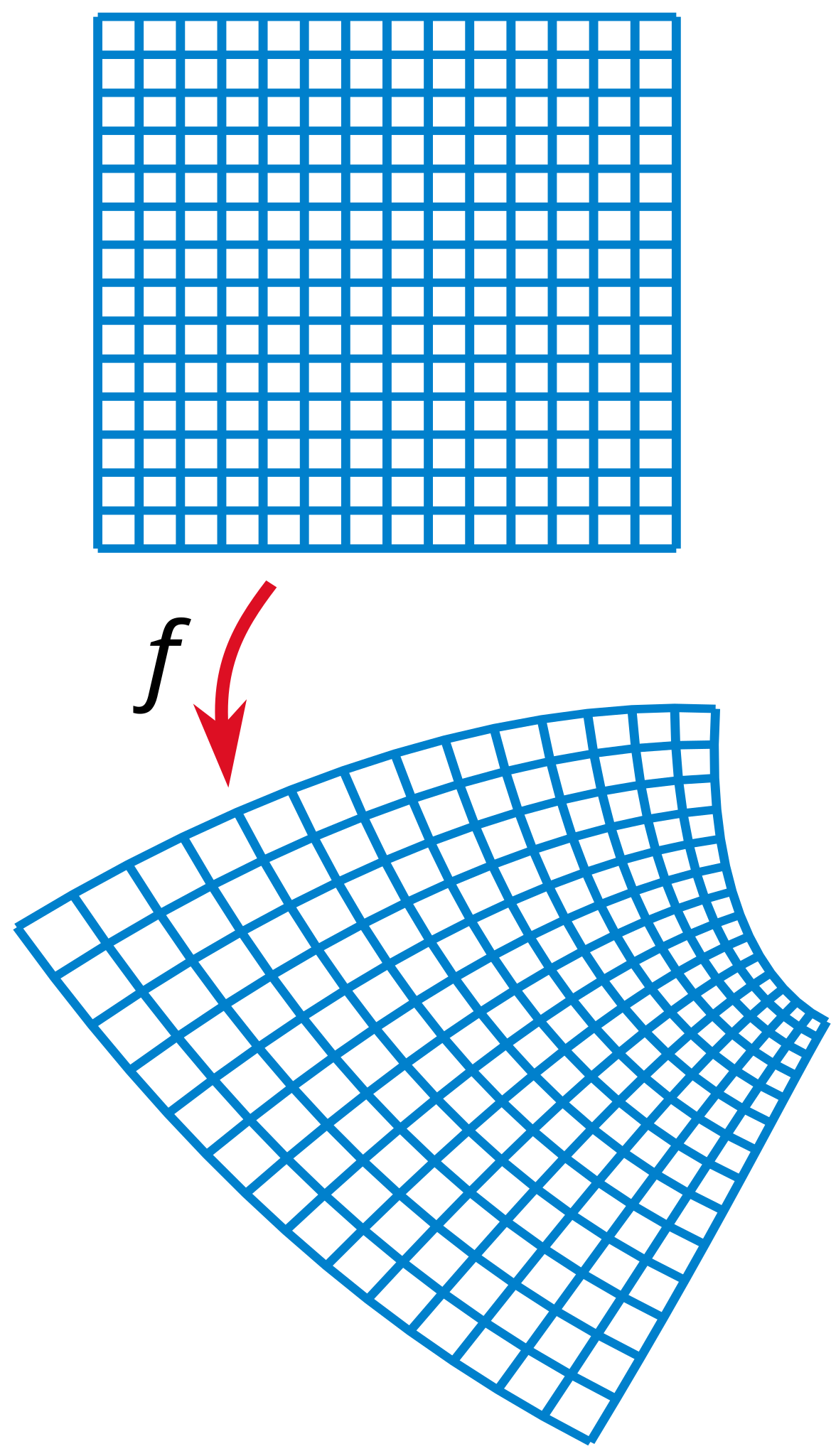
| توضیح | Illustration of a conformal map. |
| تاریخ | |
| منبع | self-made with MATLAB, tweaked in Inkscape. |
| پدیدآور | Oleg Alexandrov |
| SVG genesis | کد مبدأ این پروندهٔ گرافیک برداری مقیاسپذیر، معتبر. This file uses translateable embedded text. |
اجازهنامه
| من، دارنده حق تکثیر این اثر، این اثر را به مالکیت عمومی منتشر میکنم. این قابل اجرا در تمام نقاط جهان است. در برخی از کشورها ممکن است به صورت قانونی این امکانپذیر نباشد؛ اگر چنین است: من اجازهٔ استفاده از این اثر را برای هر مقصودی، بدون هیچگونه شرایطی میدهم، تا وقتی که این شرایط توسط قانون مستلزم نشده باشد. |
Source code (MATLAB)
% Compute the image of a rectangular grid under a a conformal map.

function main()

   N = 15; % num of grid points
   epsilon = 0.1; % displacement for each small diffeomorphism
   num_comp = 10; % number of times the diffeomorphism is composed with itself

   S = linspace(-1, 1, N);

   [X, Y] = meshgrid(S);


   % graphing settings
   lw = 1.0;

   % KSmrq's colors
   red    = [0.867 0.06 0.14];
   blue   = [0, 129, 205]/256;
   green  = [0, 200,  70]/256;
   yellow = [254, 194,   0]/256;
   white = 0.99*[1, 1, 1];

   mycolor = blue;

   % start plotting
   figno=1; figure(figno); clf;

   shiftx = 0; shifty = 0; scale = 1;
   do_plot(X, Y, lw, figno, mycolor, shiftx, shifty, scale)

   I=sqrt(-1);
   Z = X+I*Y;

   % tweak these numbers for a pretty map
   z0 = 1+ 2*I;
   z1 = 0.1+ 0.2*I;
   z2 = 0.2+ 0.3*I;
   a = 0.01;
   b = 0.02;
   shiftx = 0.1; shifty = 1.2; scale = 1.4;
   F = (Z+z0).^2 +a*(Z+z1).^3 +b*(Z+z2).^4;
   F = (1+2*I)*F;

   XF = real(F); YF=imag(F);

   do_plot(XF, YF, lw, figno, mycolor, shiftx, shifty, scale)

   axis ([-1 1.3 -2 2]); axis off;

   saveas(gcf, 'Conformal_map.eps', 'psc2');


function do_plot(X, Y, lw, figno, mycolor, shiftx, shifty, scale)
   figure(figno); hold on;

   [M, N] = size(X);

   X = X - min(min(X));
   Y = Y - min(min(Y));

   a = max(max(max(abs(X))), max(max(abs(Y))));
   X = X/a; Y = Y/a;

   X = scale*(X-shiftx);
   Y = scale*(Y-shifty);

   for i=1:N
      plot(X(:, i), Y(:, i), 'linewidth', lw, 'color', mycolor);
      plot(X(i, :), Y(i, :), 'linewidth', lw, 'color', mycolor);
   end
%   axis([-1-small, 1+small, -1-small, 1+small]);
   axis equal; axis off;
تاریخچهٔ پرونده
روی تاریخ/زمانها کلیک کنید تا نسخهٔ مربوط به آن هنگام را ببینید.
| تاریخ/زمان | بندانگشتی | ابعاد | کاربر | توضیح | |
|---|---|---|---|---|---|
| کنونی | ۲۷ ژانویهٔ ۲۰۰۸، ساعت ۲۱:۵۱ | | ۵۳۵ در ۹۳۷ (۳۴ کیلوبایت) | Oleg Alexandrov | Make arrow and text smaller |
| ۲۳ ژانویهٔ ۲۰۰۸، ساعت ۰۳:۳۶ |  | ۵۳۵ در ۹۳۷ (۳۴ کیلوبایت) | Oleg Alexandrov | {{Information |Description=Illustration of a conformal map. |Source=self-made with MATLAB, tweaked in Inkscape. |~~~~~ |Author= Oleg Alexandrov |Permission= |other_versions= }} {{PD-self}} ==Source code ([[ |
کاربرد پرونده
صفحههای زیر از این تصویر استفاده میکنند:
کاربرد سراسری پرونده
ویکیهای دیگر زیر از این پرونده استفاده میکنند:
- کاربرد در ar.wikipedia.org
- کاربرد در ba.wikipedia.org
- کاربرد در ca.wikipedia.org
- کاربرد در cbk-zam.wikipedia.org
- کاربرد در cs.wikipedia.org
- کاربرد در de.wikipedia.org
- کاربرد در de.wikiversity.org
- Holomorphie/Kriterien
- Kurs:Riemannsche Flächen (Osnabrück 2022)/Vorlesung 1
- Kurs:Riemannsche Flächen (Osnabrück 2022)/Vorlesung 1/kontrolle
- Satz über die Umkehrabbildung/Implizite Abbildung/C/Zusammenfassung/Textabschnitt
- Kurs:Funktionentheorie (Osnabrück 2023-2024)/Vorlesung 4
- Kurs:Funktionentheorie (Osnabrück 2023-2024)/Vorlesung 4/kontrolle
- کاربرد در el.wikipedia.org
- کاربرد در en.wikipedia.org
- کاربرد در es.wikipedia.org
- کاربرد در fi.wikipedia.org
- کاربرد در fr.wikipedia.org
- کاربرد در gl.wikipedia.org
- کاربرد در he.wikipedia.org
- کاربرد در hi.wikipedia.org
- کاربرد در hu.wikipedia.org
- کاربرد در hy.wikipedia.org
- کاربرد در id.wikipedia.org
- کاربرد در it.wikipedia.org
- کاربرد در ja.wikipedia.org
نمایش استفادههای سراسری از این پرونده.